Year11-MATH-2-1-3 Linear Equations and Graphs

A linear equation is an equation where the highest exponent of the variables is 1, resulting in a straight line when graphed on a coordinate plane. The most common form used in this context is the slope-intercept form:

  $y=mx+b$

Where: 

• x is the independent variable (input).
• y is the dependent variable (output).
• m is the slope or gradient, representing the constant rate of change or the “steepness” of the line. It’s calculated as the rise over the run.
• b is the y-intercept, which is the value of y when x is zero (where the line crosses the vertical axis), representing the starting or base value. 

Students learn to: 

• Develop a linear equation from a word description or given two points.
• Construct straight-line graphs, with or without technology, by finding two points or using the slope and intercept.
• Interpret the slope and intercept within the context of a practical problem (e.g., the slope might be the cost per litre of fuel, and the intercept the initial service fee).
• Solve simultaneous linear equations to find the point of intersection of two lines, which can represent a break-even point in business studies, for example. 

Trend Analysis 

Trend analysis in this context involves using linear relationships to identify and describe patterns in data and make informed predictions about future or unknown values. This is often done using real-world data plotted on a scatter plot, where a perfect straight line is unlikely due to variability. 

Key aspects include: 

• Identifying Trends: Using a trend line (also known as a line of best fit) to visually represent the general direction of the data points.
• Interpreting Slope:
  • A positive slope indicates a positive association (as x increases, y tends to increase).
  • A negative slope indicates a negative association (as x increases, y tends to decrease).
  • A slope near zero suggests no significant linear relationship.
• Linear Modelling: The process of using a linear equation to represent a real-world situation, such as modelling the distance travelled over time or population changes.
• Making Predictions: Using the equation of the trend line to estimate values within (interpolation) or sometimes beyond (extrapolation) the existing data range, while understanding the limitations and potential unreliability of extrapolating too far. 

In summary, Year 11 students move from simple algebraic manipulation of linear equations to applying these concepts to model and analyse practical situations, making predictions and interpreting the meaning of the graphs and equations in context.

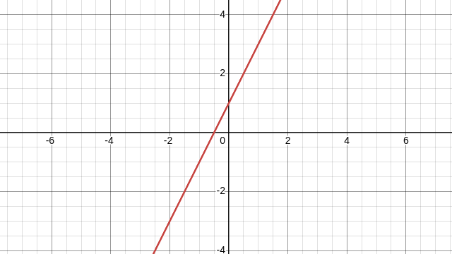
>> Example: y = 2x +1

A graph of a linear equation is a straight line, representing the relationship between variables, often shown as , where m is the slope (steepness) and is the y-intercept (where it crosses the y-axis). For example, in y = 2x + 1, the line crosses the y-axis at (0, 1) and rises 2 units for every 1 unit it moves to the right, forming a clear straight line when points like (-1, -1), (0, 1), and (1, 3) are plotted and connected.

Example:

1. Identify Slope & Y-intercept:
2. Slope ($m$): 2 (meaning ‘rise 2, run 1’).
3. Y-intercept ($c$): 1 (the point (0, 1)).

2. Plot Points (Table Method):
   • Choose x-values (e.g., -1, 0, 1).
   • Calculate y-values using the equation.
   • Points: (-1, -1), (0, 1), (1, 3).
3. Graph:
   • Plot the points on a coordinate plane.
   • Draw a straight line through them. 

Visual Representation

********************************************************************************************************************************************************

オーストラリアの11年生一般数学では、線形方程式とそのグラフのトピックで、直線グラフを用いて現実世界の実際的な状況（燃料費、人口増加、単純な運動など）をモデル化、分析、解釈し、予測を行うことに焦点を当てています。これは傾向分析の本質です。

線形方程式とグラフ

線形方程式とは、変数の最大の指数が1である方程式で、座標平面上にグラフ化すると直線になります。この文脈で最もよく使われる形式は、傾き・切片形式です。

ここで：

• x は独立変数（入力）。

• y は従属変数（出力）。

• m は傾きまたは勾配で、一定の変化率、つまり直線の「傾き」を表します。これは、上昇率を上昇率で割った値として計算されます。

• b は y 切片で、x が 0 のとき（直線が縦軸と交差する点）の y の値であり、開始値または基準値を表します。

生徒は以下のことを学びます。

• 言葉による説明または与えられた 2 点から線形方程式を立てる。

• テクノロジーの有無にかかわらず、2 点を求めるか傾きと切片を用いて直線グラフを作成する。

• 実際の問題の文脈において傾きと切片を解釈する（例：傾きは燃料 1 リットルあたりのコスト、切片は初期サービス料金）。

• 連立線形方程式を解いて 2 本の直線の交点を求める。これは、例えばビジネス研究において損益分岐点を表すことができる。

傾向分析

この文脈における傾向分析では、線形関係を用いてデータのパターンを識別・説明し、将来の値や未知の値について情報に基づいた予測を行います。これは、多くの場合、散布図にプロットされた実際のデータを用いて行われますが、変動性のために完全な直線となる可能性は低いからです。

主な側面は以下のとおりです。

• 傾向の特定：傾向線（最適適合線とも呼ばれます）を使用して、データポイントの大まかな方向性を視覚的に表します。

• 傾きの解釈：

◦ 正の傾きは正の相関を示します（x が増加すると、y も増加する傾向があります）。

◦ 負の傾きは負の相関を示します（x が増加すると、y は減少する傾向があります）。

◦ 傾きがゼロに近い場合、有意な線形関係がないことを示します。

• 線形モデリング：時間の経過に伴う移動距離や人口の変化をモデル化するなど、線形方程式を使用して現実世界の状況を表すプロセス。

• 予測：傾向線の方程式を使用して、既存のデータ範囲内（内挿）または場合によっては範囲外（外挿）の値を推定します。外挿しすぎると、限界と信頼性が低下する可能性があることを理解します。

要約すると、11 年生の生徒は、単純な代数的線形方程式の操作から、これらの概念を適用して実際の状況をモデル化および分析し、予測を行い、文脈におけるグラフと方程式の意味を解釈する段階に進みます。

>> 例: y = 2x +1

一次方程式のグラフは直線で、変数間の関係を表します。多くの場合、 と表記されます。ここで、m は傾き（勾配）、 はy切片（y軸と交わる点）です。例えば、y = 2x + 1 の場合、直線はy軸と点 (0, 1) で交わり、右に1単位移動するごとに2単位上昇します。したがって、(-1, -1)、(0, 1)、(1, 3) などの点をプロットして結ぶと、明確な直線となります。

例: y = 2x + 1

1. 傾きとy切片を特定する:

◦ 傾き ($m$): 2 (「上昇2、下降1」を意味します)。

◦ y切片 ($c$): 1 (点 (0, 1))。

2. 点のプロット（表方式）：

◦ x 値を選択します（例：-1, 0, 1）。

◦ 式を使用して y 値を計算します。

◦ 点：(-1, -1)、(0, 1)、(1, 3)。

3. グラフ：

◦ 座標平面上に点をプロットします。

◦ 点を通る直線を描きます。